by Douglas Burke on 23 October 2012
Updated October 24
Oops; I got my ACIS chips mixed up yesterday; the group is close to the boundary between the ACIS-I0 and ACIS-I2 (not ACIS-I1) chips. I have amended the text below.
Setting up
The following analysis uses CIAO version 4.4 with the latest (at the time) calibration release, namely CALDB 4.5.3
% ciaover -v
The current environment is configured for:
  CIAO        : CIAO 4.4 Tuesday, June 5, 2012
  Tools       : Package release 2  Tuesday, June 5, 2012
  Sherpa      : Package release 2  Tuesday, June 5, 2012
  Chips       : Package release 1  Friday, December 2, 2011
  Prism       : Package release 1  Friday, December 2, 2011
  Obsvis      : Package release 1  Friday, December 2, 2011
  Core        : Package release 1  Friday, December 2, 2011
  Graphics    : Package release 1  Friday, December 2, 2011
  bindir      : /export/local/ciao-4.4/bin
  Python path : CIAO

CIAO Installation: osx64
System information:
Darwin luggnagg 10.8.0 Darwin Kernel Version 10.8.0: Tue Jun  7 16:33:36 PDT 2011; root:xnu-1504.15.3~1/RELEASE_I386 i386
% check_ciao_caldb
CALDB environment variable = /export/local/ciao-4.4/CALDB
             CALDB version = 4.5.3
             release date  = 2012-10-15T16:00:00 UTC
CALDB query completed successfully.
I like to use a separate parameter file for each dataset, so I change the PFILES environment variable (using tcsh syntax):
% setenv PFILES "`pwd`/param;$ASCDS_INSTALL/param:${ASCDS_CONTRIB}/param"
% echo $PFILES
/Volumes/luggnaggraid/blog/group-data/param;/export/local/ciao-4.4/param:/export/local/ciao-4.4/contrib/param
% paccess chandra_repro
/Volumes/luggnaggraid/blog/group-data/param/chandra_repro.par
Data download
We start by downloading the data for Observation 1655:
% cd /Volumes/luggnaggraid/blog/group-data
% download_chandra_obsid 1655
Downloading files for ObsId 1655, total size is 97 Mb.

  Type     Format      Size  0........H.........1  Download Time Average Rate
  ---------------------------------------------------------------------------
  vv       pdf        34 Kb  ####################          < 1 s  692.9 kb/s
  oif      fits       23 Kb  ####################          < 1 s  549.5 kb/s
  cntr_img fits       66 Kb  ####################          < 1 s  1099.8 kb/s
  cntr_img jpg       492 Kb  ####################          < 1 s  4117.1 kb/s
  evt2     fits        3 Mb  ####################            2 s  1950.4 kb/s
  full_img fits       56 Kb  ####################          < 1 s  720.0 kb/s
  full_img jpg        74 Kb  ####################          < 1 s  1247.0 kb/s
  bpix     fits       38 Kb  ####################          < 1 s  530.2 kb/s
  fov      fits        6 Kb  ####################          < 1 s  162.1 kb/s
  eph1     fits      281 Kb  ####################          < 1 s  2809.7 kb/s
  asol     fits        5 Mb  ####################            1 s  3765.3 kb/s
  evt1     fits       42 Mb  ####################            8 s  5421.9 kb/s
  flt      fits        7 Kb  ####################          < 1 s  44.2 kb/s
  msk      fits        5 Kb  ####################          < 1 s  151.1 kb/s
  mtl      fits      921 Kb  ####################          < 1 s  1935.2 kb/s
  stat     fits      634 Kb  ####################          < 1 s  833.9 kb/s
  bias     fits      428 Kb  ####################            1 s  405.8 kb/s
  bias     fits      429 Kb  ####################          < 1 s  467.1 kb/s
  bias     fits      426 Kb  ####################          < 1 s  2842.1 kb/s
  bias     fits      420 Kb  ####################          < 1 s  1942.1 kb/s
  bias     fits      429 Kb  ####################            2 s  258.3 kb/s
  pbk      fits        4 Kb  ####################          < 1 s  87.5 kb/s
  vv       pdf        40 Mb  ####################           11 s  3895.3 kb/s
  eph1     fits       10 Kb  ####################          < 1 s  30.6 kb/s
  eph1     fits      273 Kb  ####################          < 1 s  3064.0 kb/s
  eph1     fits      249 Kb  ####################          < 1 s  2691.4 kb/s
  osol     fits      353 Kb  ####################          < 1 s  1843.1 kb/s
  aqual    fits      312 Kb  ####################          < 1 s  497.8 kb/s
  osol     fits      344 Kb  ####################          < 1 s  2718.4 kb/s
  osol     fits      329 Kb  ####################          < 1 s  1464.7 kb/s
  osol     fits      357 Kb  ####################          < 1 s  640.8 kb/s

      Total download size for ObsId 1655 = 97 Mb
      Total download time for ObsId 1655 = 30 s
and then we re-process it, to ensure that the latest calibration data is used (this repeats some of the analysis used to create the “discovery image”, but it doesn’t take too long to repeat.
% chandra_repro 1655 outdir=We can create a broad-band (0.5 to 7.0 keV) exposure-corrected image of the observation with the fluximage script, noting that we restrict the analysis to just the ACIS-I array (this is done by the [ccd_id=0:3] expression) and chose a binning of 2 ACIS pixels (so the output image has a pixel size of 2 * 0.492, or 0.984 arcseconds):
% fluximage "1655/repro/acisf01655_repro_evt2.fits[ccd_id=0:3]" qimg/ bin=2
Running fluximage
Version: 06 October 2012

Using CSC ACIS broad science energy band.
Aspect solution 1655/repro/pcadf097142619N003_asol1.fits found.
Bad pixel file 1655/repro/acisf01655_repro_bpix1.fits found.
Mask file 1655/repro/acisf01655_000N003_msk1.fits found.
PBK file 1655/repro/acisf097142234N003_pbk0.fits found.

The output images will have 1472 by 1473 pixels, pixel size of 0.984 arcsec,
    and cover x=2950.5:5894.5:2,y=2834.5:5780.5:2.

Running tasks in parallel with 4 processors.
Creating aspect histograms for obsid 1655
Creating 4 instrument maps for obsid 1655
Creating 4 exposure maps for obsid 1655
Exposure map limits: 0.000000e+00, 5.512396e+06
Writing exposure map to qimg/2_broad.expmap
Exposure map limits: 0.000000e+00, 5.325326e+06
Writing exposure map to qimg/0_broad.expmap
Exposure map limits: 0.000000e+00, 5.378100e+06
Writing exposure map to qimg/1_broad.expmap
Exposure map limits: 0.000000e+00, 5.496100e+06
Writing exposure map to qimg/3_broad.expmap
Combining 4 exposure maps for obsid 1655
Thresholding data for obsid 1655
Exposure-correcting image for obsid 1655

The following files were created:

 The clipped counts image is:
     qimg/broad_thresh.img

 The clipped exposure map is:
     qimg/broad_thresh.expmap

 The exposure-corrected image is:
     qimg/broad_flux.img
Which we view using ChIPS:
% chips
-----------------------------------------
Welcome to ChIPS: CXC's Plotting Package
-----------------------------------------
CIAO 4.4 ChIPS version 1 Tuesday, June 5, 2012

chips-1> from crates_contrib.all import *
chips-2> cr = read_file("qimg/broad_flux.img")
chips-3> smooth_image_crate(cr, "gauss", 3)
chips-4> scale_image_crate(cr, "log10")
Warning: divide by zero encountered in log10
chips-5> add_window(8, 8, "inches")
chips-6> add_image(cr)
chips-7> set_image(['threshold', [-8,-6.5]])
chips-8> set_image(['threshold', [-8.5,-6.5]])
chips-9> set_image(['depth', 50])
chips-10> set_xaxis(['tickformat', '%ra'])
chips-11> set_yaxis(['tickformat', '%dec'])
chips-12> set_axis(['*.size', 18])
chips-13> set_axis(['*.size', 16])
chips-14> set_plot_title('0.5-7.0 keV, ObsId 1655')
chips-15> set_frame(['bgcolor', 'black'])
chips-16> set_axis(['*.color', 'white'])
chips-17> set_plot(['title.color', 'white', 'title.size', 18])
chips-18> from chips_contrib.all import *
chips-19> add_fov_region('1655/repro/acisf01655_000N003_fov1.fits[ccd_id=0:3]')
chips-20> set_region('all', ['fill.style', 'empty'])
chips ERROR: The fill style value (empty) must be one of [nofill, solidfill, updiagonal, downdiagonal, horizontal, vertical, crisscross, brick, grid, hexagon, polkadot, flower, userfill1, userfill2, userfill3]
chips-21> set_region('all', ['fill.style', 'nofill'])
chips-22> print_window('qimg.png')
chips-23> quit()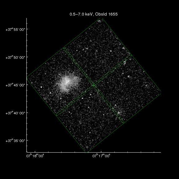
Quick look at the broad-band data; the green rectangles show the outline of each of the ACIS-I chips
As can be seen the putative group, which is at 07h16m44. 3s and 37o 39’ 55", is very close to the boundaries between two chips (in this case ACIS-I0 and ACIS-I1 ACIS-I2; the ACIS Instrument Information page has more information on the layout and details of the ACIS detector).
It’s time to go home for the day; hopefully I’ll get time tomorrow to extract a spectrum of the point source and do some simple analysis on the extended emission.
