by Douglas Burke on 24 October 2012
Before extracting spectra, let’s do some sanity checks.
Background flares
Chandra observations can be affected by “background flares”; that is periods of time when the particle background is not constant (for more information see the ACIS Background Memos page from the Calibration team). This flaring need not be a problem for analysis of bright point sources, but as we are interested in faint, extended emission it is worth checking the high-energy light curve for signs of variability.
Since ACIS has essentially no sensitivity above 9 keV, we chose to look at the 10 to 12 keV data, which is created by the particle background, for the ACIS-I0 and ACIS-I2 chips (these are the two that lie close to the group).
% punlearn dmextract
% dmextract "1655/repro/acisf01655_repro_evt2.fits[ccd_id=0,2,energy=10000:12000][bin time=::500]" qbg.lc opt=ltc1
% dmlist qbg.lc cols

--------------------------------------------------------------------------------
Columns for Table Block LIGHTCURVE
--------------------------------------------------------------------------------

ColNo  Name                 Unit        Type             Range
   1   TIME_BIN             channel      Int4           1:45                 S/C TT corresponding to mid-exposure
   2   TIME_MIN             s            Real8          97141592.4202499986: 97163977.9086109996 Minimum Value in Bin
   3   TIME                 s            Real8          97141592.4202499986: 97163977.9086109996 S/C TT corresponding to mid-exposure
   4   TIME_MAX             s            Real8          97141592.4202499986: 97163977.9086109996 Maximum Value in Bin
   5   COUNTS               count        Int4           -                    Counts
   6   STAT_ERR             count        Real8          0:+Inf               Statistical error
   7   AREA                 pixel**2     Real8          -Inf:+Inf            Area of extraction
   8   EXPOSURE             s            Real8          -Inf:+Inf            Time per interval
   9   COUNT_RATE           count/s      Real8          0:+Inf               Rate
  10   COUNT_RATE_ERR       count/s      Real8          0:+Inf               Rate Error

--------------------------------------------------------------------------------
World Coord Transforms for Columns in Table Block LIGHTCURVE
--------------------------------------------------------------------------------

ColNo    Name
2:    DT_MIN               = +0 [s] +1.0 * (TIME_MIN  -97141842.420250)
3:    DT                   = +0 [s] +1.0 * (TIME  -97141842.420250)
4:    DT_MAX               = +0 [s] +1.0 * (TIME_MAX  -97141842.420250)
Plotting up the count rate gives us the following (since I use the “virtual” columns DT_MIN and DT_MAX to plot up the time since the start of the observation, I have to work around a bug in Crates in CIAO 4.4 which means the data needs to be re-shaped to exclude garbage values):
% chips
-----------------------------------------
Welcome to ChIPS: CXC's Plotting Package
-----------------------------------------
CIAO 4.4 ChIPS version 1 Tuesday, June 5, 2012

chips-1> cr = read_file("qbg.lc")
chips-2> xlo = cr.get_column("dt_min").values
chips-3> xhi = cr.get_column("dt_max").values
chips-4> xlo.shape
         (45, 2)
chips-5> xlo = xlo.reshape(45*2)[:45]
chips-6> xhi = xhi.reshape(45*2)[:45]
chips-7> y = cr.get_column("count_rate").values
chips-8> dy = cr.get_column("count_rate_err").values
chips-9> add_window(8, 5, "inches")
chips-10> add_histogram(xlo, xhi, y, dy)
chips-11> set_plot_xlabel(r"\Delta T (s)")
chips-12> set_plot_ylabel("Count rate (s^{-1])")
chips-13> set_plot_title("10 - 12 keV lightcurve for ACIS-I0,I2")
chips-14> set_axis("all", ["label.size", 20, "ticklabel.size", 16])
chips-15> set_plot(["title.size", 20])
chips-16> set_plot_ylabel("Count rate (s^{-1})")
chips-17> print_qindow('qbg.png')
NameError: name 'print_qindow' is not defined
chips-18> print_window('qbg.png')
chips-19> quit()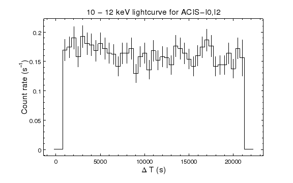
The light curve of the 10 to 12 keV particles in the ACIS-I0 and I2 chips looks consistent. This can be compared to the background lightcurve created below from source-free regions of the detector.
Source Detection
Using the binned-by-2 data from yesterday, let’s get a source list since we can use it as a more accurate source location, and for identifying a source-free region for analysis later on.
For this I shall use the wavdetect tool provided in CIAO, roughly following the running wavdetect thread.
% cd qimg
% punlearn mkspfmap
% mkpsfmap broad_thresh.img broad.psfmap 1.4967 0.393
The PSF map isn’t interesting visually - it basically shows that the PSF increases as you move further away from the aimpoint - but we can get an estimate for the PSF size at the location of the group:
% dmstat "broad.psfmap[sky=circle(7:16:44.3,37:39:55,2"")]" cen- sig-
broad.psfmap[arcsec]
    min:	3.2938494682 	      @:	( 4961.5 3699.5 )
    max:	3.3122434616 	      @:	( 4963.5 3697.5 )
   mean:	3.3030492663
    sum:	13.212197065
   good:	4
   null:	5
So at 1.5 keV the PSF size (at which the enclosed energy fraction is 39.3 percent) is about 3.3 arcsec.
Since I am using the whole ACIS-I array here, I include the exposure map to reduce problems at the gaps between the chips, and use a range of scales to better model the extended emission from the cluster (even though we are not interested in this emission here). Note that I do not go above a scale size of 64 to avoid a known bug with large scale sizes in CIAO 4.4; for the analysis presented here, which does not use data near the cluster, the lack of these large scales is not a problem.
% punlearn wavdetect
% wavdetect broad_thresh.img src.fits scell.fits wimg.fits wbkg.fits \
      scales="2 4 8 16 32 64" psffile=broad.psfmap regfile=src.reg \
      expfile=broad_thresh.expmap
% ds9 broad_flux.img -region ../1655/repro/acisf01655_000N003_f1.fits \
      -region color white -region src.fits -log -pan to 4950 3700 \
      wimg.fits -cmap b -region color blue -region width 2 \
      -region src.fits -scale mode 99.5 -pan to 4950 3700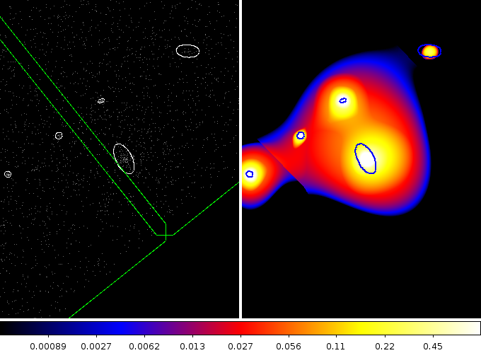
The white ellipses on the left/blue on the right show the sources detected by wavdetect. The image on the left is the broad-band (0.5 to 7.0 keV) image, with green lines indicating the chip edges, and the image no the right is the wavelet-reconstructed source image, shown with a log scale to highlight the extended emission around the source of interest. I was slightly surprised to see this extended emission, but it’s a nice confirmation that I am not imagining things. Since the source lies right next to the chip edge I am not going to use this reconstruction for charecterising the source emission.
Looking at the source list, restricting to close to the group, I find three sources - since
% dmlist "src.fits[pos=circle(4950,3700,250)]" countsand some of the source properties are
% dmlist "src.fits[pos=circle(4950,3700,250)][cols pos,ra,dec,src_significance,net_counts,net_counts_err,r,rotang,psfratio]" data

--------------------------------------------------------------------------------
Data for Table Block SRCLIST
--------------------------------------------------------------------------------

ROW    POS(X,Y)                                 RA                   DEC                  SRC_SIGNIFICANCE     NET_COUNTS           NET_COUNTS_ERR       R[2]                                     ROTANG               PSFRATIO

     1 (     4778.0714285714,     3766.2142857143)       109.2164132207        37.6746305192         4.9632539749        12.4653091431         3.7416591644 [       10.0189418793         9.7587423325]        17.4122447968     0.73306226730347
     2 (     4962.7345679012,     3700.7592592593)       109.1845457936        37.6656490623        15.8159770966        70.0091934204         9.0000047684 [       45.8681144714        22.9423046112]       117.1847610474         1.6089938879
     3 (     4898.2777777778,     3864.8333333333)       109.1956322045        37.6880859683        12.2616348267        32.9132995605         5.9160809517 [        9.3221349716         5.0649147034]        18.7779579163     0.43097385764122
so the source location (the second row in the table) is RA=109.1845457936 degrees and Dec=37.6656490623 which we can convert into sexagessimal notation:
% chips
-----------------------------------------
Welcome to ChIPS: CXC's Plotting Package
-----------------------------------------
CIAO 4.4 ChIPS version 1 Tuesday, June 5, 2012

chips-1> import coords.format as fmt
chips-2> fmt.deg2ra(109.1845457936, ':')
         '7:16:44.290990464'
chips-3> fmt.deg2dec(37.6656490623, ':')
         '37:39:56.33662428'
chips-4> quit()
so RA=7h 16m 44. 3s and Dec= + 37o 39’ 56", and we can use dmcoords to find it’s location on the ACIS-I array:
% dmcoords broad_flux.img ../1655/primary/pcadf097142619N003_asol1.fits
dmcoords>: sky 4962.73 3700.76
(RA,Dec):     07:16:44.291    +37:39:56.33
(RA,Dec):      109.18455       37.66565 deg
THETA,PHI          7.809'        206.76 deg
(Logical):        1006.61        433.63
SKY(X,Y):         4962.73       3700.76
DETX,DETY         3246.13       3667.75
CHIP ACIS-I0       993.50        220.96
TDET              3281.96       4138.50
dmcoords>: quit
A source-free light curve
Now we have a source list we can try creating a source-free lightcurve. First we need to increase the radii of each source to make sure we are excluding as much of the source signal as possible whilst retaining some background; for this I use a scaling factor of 3, which I’ve found to give good results in the past:
% punlearn dmtcalc
% dmtcalc src.fits src.excl3.fits expr="R=R*3"
% dmstat src.fits"[cols r]" sig-
R[pixel]
    min:	[ 2.6729438305 1.8822516203 ] 	      @:	[ 13 13 ]
    max:	[ 47.656509399 28.958713531 ] 	      @:	[ 47 52 ]
   mean:	[ 15.450465941 9.6179984495 ]
    sum:	[ 942.4784224 586.69790542 ]
   good:	[ 61 61 ]
   null:	[ 0 0 ]

% dmstat src.excl3.fits"[cols r]" sig-
R
    min:	[ 8.0188312531 5.6467547417 ] 	      @:	[ 13 13 ]
    max:	[ 142.9695282 86.876144409 ] 	      @:	[ 47 52 ]
   mean:	[ 46.351397655 28.853995456 ]
    sum:	[ 2827.435257 1760.0937228 ]
   good:	[ 61 61 ]
   null:	[ 0 0 ]
Now we move back up a level and create a filtered copy of the event file which we can use to extract a light curve.
% cd ..
% dmcopy 1655/repro/acisf01655_repro_evt2.fits"[ccd_id=0,2,energy=500:7000]" ccd02.fits
% dmcopy ccd02.fits"[exclude sky=region(qimg/src.excl3.fits)]" tmp.fits
% ds9 tmp.fits -bin factor -bin about 4700 3900 -smooth -cmap b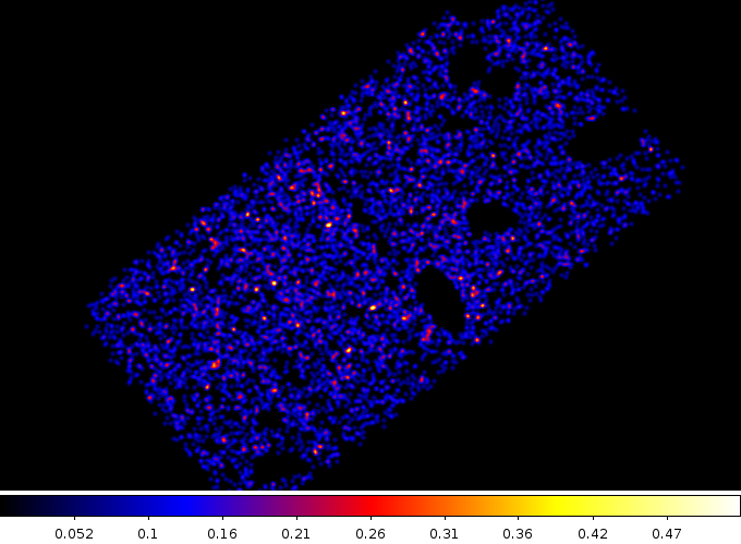
The 0.5 to 7.0 keV source-free emission from ACIS-I0 and ACIS-I2. It is likely that the exclusion region around the group should have been larger, but overall this image looks quite flat.
% punlearn dmextract
% dmextract "ccd02.fits[exclude sky=region(qimg/src.excl3.fits)][bin time=::500]" bg.lc opt=ltc1
% chips
-----------------------------------------
Welcome to ChIPS: CXC's Plotting Package
-----------------------------------------
CIAO 4.4 ChIPS version 1 Tuesday, June 5, 2012

chips-1> add_window(8, 6, 'inches')
chips-2> make_figure('bg.lc[cols time,count_rate,count_rate_err]')
chips-3> set_axis(['ticklabel.size', 16, 'label.size', 20])
chips-4> set_plot_title('0.5 - 7.0 keV background for ACIS I0 & I2')
chips-5> set_plot(['title.size', 20])
chips-6> print_window('bg.lc.png')
chips-7> quit()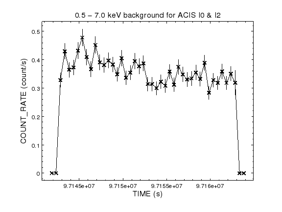
The backgronud light curve shows a similar shape to the particle flux; it is perhaps slightly-higher at the start of the observation and levels off half-way through, but the change is small, a by-eye estimate suggests a change of at most 0.05 counts s − 1, so for now I shall use all the data rather than trying to time filter it to remove background flares.
A radial profile of the group
We canuse the exposure-corrected image to get a quick look at the radial profile of the source using dmextract:
% cd qimg
% punlearn dmextract
% dmextract broad_flux.img"[bin sky=annulus(4962.7,3700.8,0:200:2)]" qprof.fits opt=generic
% dmtcalc qprof.fits qprof2.fits expr="RMID=(R[0]+R[1])/2"
% chips
-----------------------------------------
Welcome to ChIPS: CXC's Plotting Package
-----------------------------------------
CIAO 4.4 ChIPS version 1 Tuesday, June 5, 2012

chips-1> add_window(8, 6, 'inches')
chips-2> add_curve('qprof2.fits[cols rmid,sur_bri]')
chips-3> log_scale(Y_AXIS)
chips-4> set_curve(['symbol.style', 'none'])
chips-5> set_plot_xlabel("Radius (pixels)')
------------------------------------------------------------
   File "<ipython console>", line 1
     set_plot_xlabel("Radius (pixels)')
                                      ^
SyntaxError: EOL while scanning string literal

chips-6> set_plot_xlabel("Radius (pixels)")
chips-7> set_plot_ylabel("photon cm^{-2} s^{-1} pixel^{-1}")
chips-8> set_axis('all', ['ticklabel.size', 16, 'label.size', 20])
chips-9> set_yaxis(['offset.perpendicular', 60])
chips-10> set_plot_title('Radial profile of group candidate (0.5 to 7.0 keV)')
chips-11> set_plot(['title.size', 20])
chips-12> print_window('qprof.png')
chips-13> quit()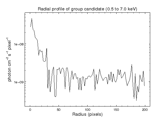
The radial profile shows obvious emission out to ∼ 30 pixels, which is ∼ 15 arcsec, and possible emission out to ∼ 100 pixels, although that could just be me reading too much into the data. A proper analysis would use the counts image, with the chip edges and other sources excluded from the profile. Note that the nearest two sources in the wavdetect output are ∼ 175 and ∼ 195 pixels away.
