by Douglas Burke on 25 October 2012
Today I don’t have a lot of time, so let’s check the X-ray emission against existing observations.
2MASS
Using the Interactive 2MASS Image Service, I have downloaded a 600 arcsec cutout in the Ks band from the All-Sky Release Survey for the position 7h 16m 44. 3s + 37o 39’ 56", which is shown below. The Data Tag for this data set is ADS/IRSA.2mass_im#2012/1025/065751_17093.
% dmlist aK_asky_980413n0070197.fits cols

--------------------------------------------------------------------------------
Columns for Image Block PRIMARY
--------------------------------------------------------------------------------

ColNo  Name                 Unit        Type             Range
   1   PRIMARY[452,387]                  Real4(452x387) -Inf:+Inf

--------------------------------------------------------------------------------
Physical Axis Transforms for Image Block PRIMARY
--------------------------------------------------------------------------------

Group# Axis#
   1   1,2    POS(X) = (#1)
                 (Y)   (#2)

--------------------------------------------------------------------------------
World Coordinate Axis Transforms for Image Block PRIMARY
--------------------------------------------------------------------------------

Group# Axis#
   1   1,2    EQPOS(RA ) = (+109.2219) +SIN[(-0.000277778)* ROT(+0.0025 deg)* (POS(X)-(+196.50))]
                   (DEC)   (+37.5473 )      (+0.000277778)                    (   (Y) (-124.50))
Here we display the 2MASS Ks band image with ChIPS and then overlay the contours showing the Chandra emission. The contours were created by ds9,
% ds9 qimg/broad_flux.img -log -smooth -pan to 4960 3700 -zoom 2using the following levels, and a smoothing scale of 3. The output was saved to qimg/group.con and then used in ChIPS below. I had aimed to use the add_ds9_contours routine but this didn’t work, so I ended up using read_ds9_contours to read in the data, then a quick spatial filter to find those contours near the group, and then display each of these as a curve (I should really have also added in a check on the Declination, not just the Right Ascension to save a little work by the computer):
% cat qimg/group.lev
0
3.75e-08
7.5e-08
1.125e-07
1.5e-07
% chips
-----------------------------------------
Welcome to ChIPS: CXC's Plotting Package
-----------------------------------------
CIAO 4.4 ChIPS version 1 Tuesday, June 5, 2012

chips-1> add_window(8, 7, 'inches')
chips-2> make_figure('aK_asky_980413n0070197.fits', 'image')
chips-3> set_image(['threshold', [300,320]])
chips-4> from coords.format import *
chips-5> ra = ra2deg('7 16 44.3')
chips-6> dec = dec2deg('37 39 56')
chips-7> ra
         109.18458333333334
chips-8> dec
         37.66555555555556
chips-9> panto(ra, dec)
chips-10> zoom(5)
chips-11> zoom(0.8)
chips-12> zoom(0.5)
chips-13> zoom(1.2)
chips-14> set_image(['depth', 50])
chips-15> from crates_contrib.utils import *
chips-16> (xs, ys) = read_ds9_contours('qimg/group.con')
chips-17> cs = [(x,y) for (x,y) in zip(xs,ys)
          if np.abs(x[0] - ra) < 0.01]
chips-18> len(cs)
          9
chips-19> for (x,y) in cs:
              add_curve(x,y,['line.color','green','symbol.style','none'])


chips-20> delete_curve('all')
chips-21> cs = [(x,y) for (x,y) in zip(xs,ys)
          if np.abs(x[0] - ra) < 0.05]
chips-23> len(cs)
          71
chips-24> for (x,y) in cs:
    add_curve(x,y,['line.color','green','symbol.style','none'])


chips-26> zoom(0.9)
chips-27> print_window('2mass-overlay.png')
chips-28> quit()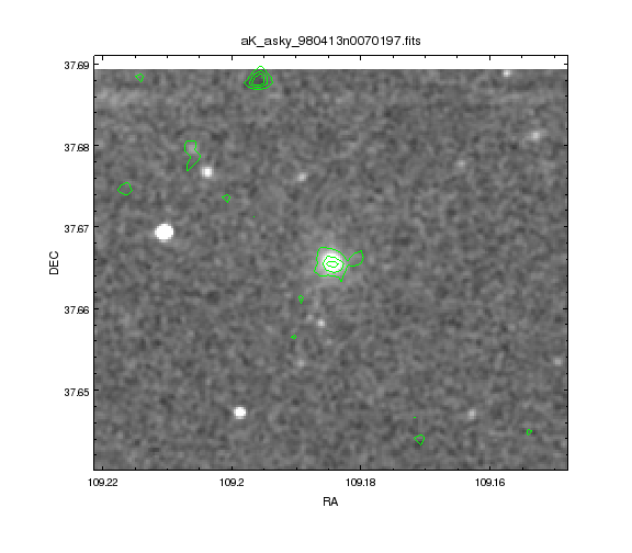
Chandra emission (in green contours) overlain on the 2MASS Ks band image, showing that the source we are interested in is spatially associated with the galaxy 2MASX J07164427+3739556. Note that many of the small blobs of emission just to the East of this source look to be noise, due to the ACIS chip edge.
Radio
The NED search shows that there is also radio emission associated with this source, NVSS J071643+373957. Using the ‘Retrieve NVSS Image’ from this page returns a 15 arcminute FITS image:
% dmlist nvss.fits cols

--------------------------------------------------------------------------------
Columns for Image Block PRIMARY
--------------------------------------------------------------------------------

ColNo  Name                 Unit        Type             Range
   1   PRIMARY[61,61,1,1]   JY/BEAM      Real4(61x61x1x1) -Inf:+Inf

--------------------------------------------------------------------------------
Physical Axis Transforms for Image Block PRIMARY
--------------------------------------------------------------------------------

Group# Axis#
   1   1,2    POS(X) = (#1)
                 (Y)   (#2)
   2   3      Z                    = #3
   3   4      #AXIS4               = #4

--------------------------------------------------------------------------------
World Coordinate Axis Transforms for Image Block PRIMARY
--------------------------------------------------------------------------------

Group# Axis#
   1   1,2    EQPOS(RA ) = (+109.1846) +SIN[(-0.0042)* (POS(X)-(+31.0))]
                   (DEC)   (+37.6656 )      (+0.0042)  (   (Y) (+31.0))
   2   3      STOKES               = Z
   3   4      FREQ                 = +1.4E+09  +100000000.0 * (#AXIS4  -1.0)
Fortunately, this time we can use add_ds9_contours:
% chips
-----------------------------------------
Welcome to ChIPS: CXC's Plotting Package
-----------------------------------------
CIAO 4.4 ChIPS version 1 Tuesday, June 5, 2012

chips-1> add_window(8, 8, 'inches')
chips-2> make_figure('nvss.fits', 'image')
chips-3> set_image(['depth', 50])
chips-4> from chips_contrib.utils import *
chips-5> add_ds9_contours('qimg/group.con')
chips-6> set_curve(['thickness', 2])
chips ERROR: Invalid ChipsCurve attribute 'thickness' in list.
chips-7> set_curve(['width', 2])
chips ERROR: Invalid ChipsCurve attribute 'width' in list.
chips-8> set_curve(['line.thickness', 2])
chips-9> zoom(2)
chips-10> print_window('nvss-overlay.png')
chips-11> quit()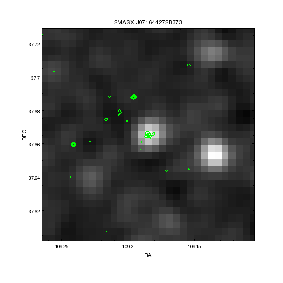
The image shown here covers a larger area than the 2MASS one above. Fortunately there is also VLA FIRST data for this field, as shown below.
If you go to the VLA FIRST archive page you can use the image cut-out service to find the FIRST data for this area (the advantage over the NVSS data shown above is the significantly better spatial resolution). I retrieved a 10 arcminute image centered on the group, which was called J071644+373956.fits but I have renamed first.fits:
% chips
-----------------------------------------
Welcome to ChIPS: CXC's Plotting Package
-----------------------------------------
CIAO 4.4 ChIPS version 1 Tuesday, June 5, 2012

chips-1> add_window(8,8,'inches')
chips-2> make_figure('aK_asky_980413n0070197.fits', 'image')
chips-3> set_image(['depth', 50, 'threshold', [300,310]])
chips-4> set_image(['depth', 50, 'threshold', [300,320]])
chips-5> add_contour('nvss.fits')
chips-6> get_contour().levels
         [0.0, 0.002, 0.004, 0.006, 0.008]
chips-7> set_contour(['levels', [0.002,0.004,0.006,0.008]])
chips-8> panto(109.17,37.66)
chips-9> zoom(2)
chips-10> add_contour('first.fits', ['color', 'cyan'])
chips-11> get_contour().levels
          [0.0, 0.002, 0.004, 0.006]
chips-12> set_contour(['levels', [0.002,0.004,0.006,0.008]])
chips-13> from crates_contrib.utils import *
chips-14> (xs,ys) = read_ds9_contours('qimg/group.con')
chips-15> ci = ChipsCurve()
chips-16> ci.line.color = 'green'
chips-17> ci.symbol.style = 'none'
chips-18> for (x,y) in zip(xs,ys):
              if (np.abs(x[0]-109.17)>0.6) or (np.abs(y[0]-37.66)>0.6):
                  continue

              add_curve(x, y, ci)


chips-19> from chips_contrib.regions import *
chips-20> add_fov_region('1655/repro/acisf01655_000N003_fov1.fits[ccd_id=0]')
chips-21> panto(109.17,37.66)
chips-22> zoom(2)
chips-23> zoom(2)
chips-24> zoom(0.75)
chips-25> set_region(['opacity', 0.2])
chips-26> print_window('radio-comparison.png')
chips-27> quit()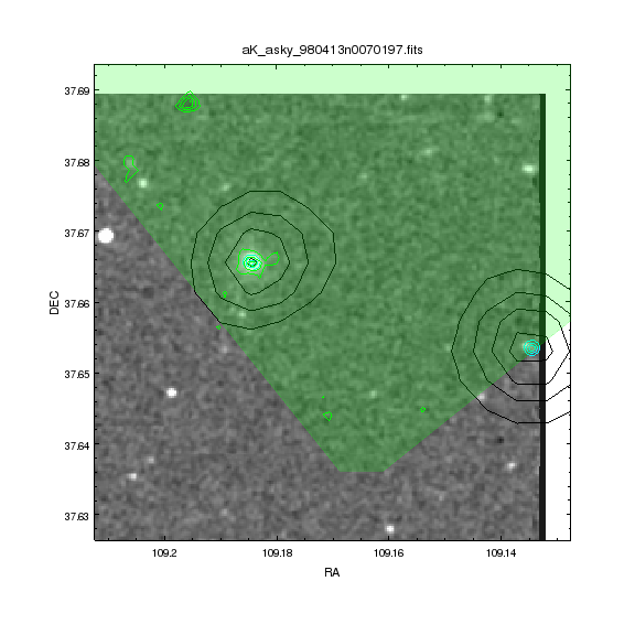
The image is the 2MASS Ks band data with three contours: X-ray (green); Radio, NVSS (black); and Radio, FIRST (cyan). The light-green shaded region shows the coverage of the ACIS-I0 chip, showing that the second radio source, to the East of the group, is right on the edge of the chip, and so may well not be detected. There is a fainter Ks band source (than the group galaxy) at this location; it just may be somewhat obscured by the contours for the radio data.
The second radio source has a position - estimated by eye using the FIRST data - of 7h 16m 32. 3s + 37o 29’ 13" - which NED identifies as NVSS J071632+373912, a source provisionally associated with the 2MASS galaxy 2MASX J07163136+3739113. Perhaps this galaxy has a similar redshift to 2MASX J07164427+3739556 (z = 0. 069), and so is associated with it?
What does this tell us?
Well, the X-ray emission is extremely likely to be associated with the galaxy which we see in the optical and near-IR. This galaxy is nearby - it has a redshift of z = 0.069, or 20708 km/s, which means that it is unassociated with the cluster target of the Chandra observation (which has a redshift of z=0.55). The X-ray emission appears faint, but extended, which is unlikely just to be the halo of the galaxy but instead the hot gas surrounding a group of galaxies (or at least that’s my hope). One way to test this is to extract the X-ray spectrum of this emission and see if it is well fit by a thermal plasma model and, if so, what is its temperature. If the system is relaxed - i.e. it has not been perturbed recently by a merger or some form of outflow from the galaxy, so that the gas traces out the gravitational potential - then the gas temperature is a good indicator of the total mass of the system. One possible fly in the ointment is that the radio emission indicates that there may be some non-thermal processes going on, which could contribute to the X-ray spectrum and so make it hard to measure any galaxy or group emission accurately.
