by Douglas Burke on 26 October 2012
So far I’ve spent too long trying to get previous/next links to appear in this blog, so let’s try and improve things and do some science.
First: where is the center of the group in chip coordinates again? I use the dmcoords tool to convert from the celestial coordinates of the source to SKY and CHIP coordinates (I use the non-interactive version just to be fancy). Now, because of the dither pattern made by Chandra during the observation there is no one position on the detector that matches the sky coordinate, but the values below are a good indicator.
% punlearn dmcoords
% dmcoords qimg/broad_thresh.img 1655/repro/pcadf097142619N003_asol1.fits \
           ra='7 16 44.3' dec='37 39 56' option=cel
% pget dmcoords x
4962.518225022578
% pget dmcoords y
3700.074715299584
% pget dmcoords chip_id
0
% pget dmcoords chipx
994.0953131998009
% pget dmcoords chipy
220.554982740513
Looking at the chip coordinates for ACIS-I0, we get
% ds9 ccd02.fits -bin filter 'ccd_id=0' -bin cols chipx chipy \
      -bin about 512 512 -zoom 0.5 -smooth -smooth radius 4 \
      -cmap b -saveimage png chip0.png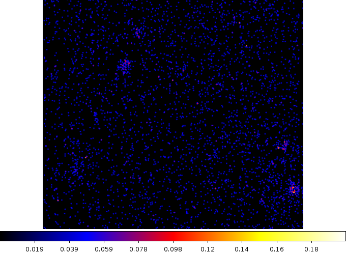
The 0.5 to 7.0 keV data for ACIS-I0 displayed in chip coordinates; the group is at (994,221), with (1,1) being the bottom-left pixel and (1024,1024) the top-right pixel, which makes it the emission in the bottom-right of the image.
Spectral extraction
I created source and background regions by eye, to give:
% cat qspec/src.reg
circle(4962.7,3700.8,20)
% cat qspec/bg.reg
circle(5146.5,4166.5,280)-ellipse(5142.9,4005.8,50,30,175)-ellipse(5025.3,4346.8,40,17,5)
These regions are based on the source detection results from Wednesday, where I have changed the source shape (from elliptical to circular and reduced the aperture size slightly) and the background region is a reasonable fraction of the ACIS-I0 chip without having to exclude too many sources. I took care to make sure that all the regions are on the same chip, but I did not bother to ensure that the background region fell on the same node as the source region (which I could have done, I just forgot, because I wanted to make sure I picked a large region for estimating the background).
% ds9 ccd02.fits -log -cmap b -region qimg/src.reg \
      -bin about 5060 4080 -bin factor 4 -zoom 2
... then qspec/src.reg and qspec/bg.reg are loaded from within ds9 and
... set to being drawn in white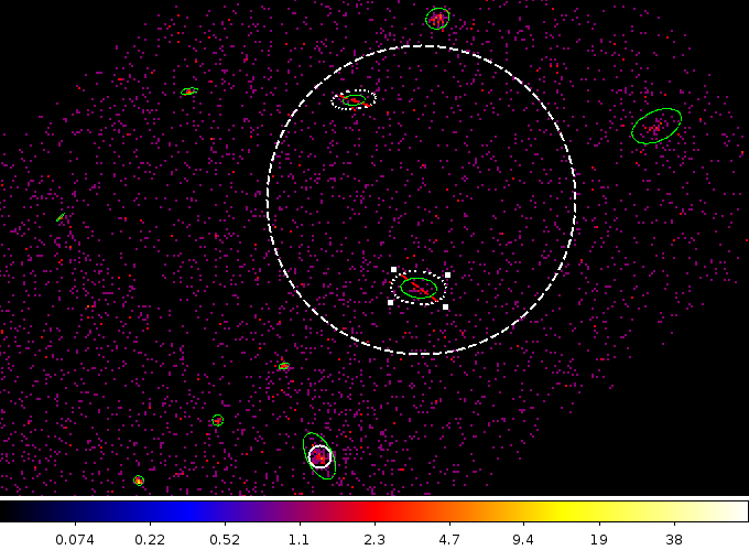
The green regions show the output from wavdetect, the solid white is the region I have selected for the initial source extraction (qspec/src.reg) and the dotted white is the background region (qspec/bg.reg), which excludes two sources using regions slightly-larger than the wavdetect output.
A quick look at the source counts in these regions, using dmstat, gives
% dmstat qimg/broad_thresh.img"[sky=region(qspec/src.reg)]" cen-
EVENTS_IMAGE
    min:	0 	      @:	( 4957.5 3681.5 )
    max:	2 	      @:	( 4959.5 3699.5 )
   mean:	0.20125786164
  sigma:	0.43840583441
    sum:	64
   good:	318
   null:	123
% dmstat qimg/broad_thresh.img"[sky=region(qspec/bg.reg)]" cen-
EVENTS_IMAGE
    min:	0 	      @:	( 5123.5 3887.5 )
    max:	2 	      @:	( 5049.5 3909.5 )
   mean:	0.014901436686
  sigma:	0.1222565917
    sum:	892
   good:	59860
   null:	18540
so the background level within the source is small (this is for the 0.5 to 7.0 keV band):
% chips -n
chips-1> 892 * 318 / 59860.0
         4.738656866020715
chips-2> quit()
So, there’s about 59 source counts and 5 background counts in the source region.
Since there are a lot of parameters to the specextract script, I am going to set the separately using pset, rather than give them all on the command line when calling specextract. I chose to use the “extended source” analysis version - that is set weight=yes and correct=no - since I am using a relatively large aperture of r=20 pixels (although the PSF is significantly larger at this off-axis angle than at the aimpoint, as discussed on Wednesday, it seems better to use the extended-source approach here):
% punlearn specextract
% pset specextract infile=1655/repro/acisf01655_repro_evt2.fits"[sky=region(qspec/src.reg)]"
% pset specextract bkgfile=1655/repro/acisf01655_repro_evt2.fits"[sky=region(qspec/bg.reg)]"
% pset specextract asp=1655/repro/pcadf097142619N003_asol1.fits
% pset specextract pbkfile=1655/repro/acisf097142234N003_pbk0.fits
% pset specextract mskfile=1655/repro/acisf01655_000N003_msk1.fits
% pset specextract badpixfile=1655/repro/acisf01655_000N003_bpix1.fits
% specextract outroot=qspec/group grouptype=NONE
Source event file(s) (1655/repro/acisf01655_repro_evt2.fits[sky=region(qspec/src.reg)]):
Should response files be weighted? (yes):
Apply point source aperture correction to ARF? (no):
Combine ungrouped output spectra and responses? (no):
Background event file(s) (1655/repro/acisf01655_repro_evt2.fits[sky=region(qspec/bg.reg)]):
Create background ARF and RMF? (yes):
Source aspect solution or histogram file(s) (1655/repro/pcadf097142619N003_asol1.fits):
pbkfile input to mkwarf (1655/repro/acisf097142234N003_pbk0.fits):
mskfile input to mkwarf (1655/repro/acisf01655_000N003_msk1.fits):

Running: specextract
  Version:    14 February 2012

Setting bad pixel file for item 1 of 1 in input list


Extracting src spectra for item 1 of 1 in input list


Creating src ARF for item 1 of 1 in input list


Creating src RMF for item 1 of 1 in input list


Using mkacisrmf...

Updating header of qspec/group.pi with RESPFILE and ANCRFILE keywords.

Setting bad pixel file for item 1 of 1 in input list


Extracting bkg spectra for item 1 of 1 in input list


Creating bkg ARF for item 1 of 1 in input list


Creating bkg RMF for item 1 of 1 in input list


Using mkacisrmf...

Updating header of qspec/group_bkg.pi with RESPFILE and ANCRFILE keywords.
Updating header of qspec/group.pi with BACKFILE keyword.
Unfortunately this took a while since the calculation of the weighted response for the background region is time consuming, as it is a relatively large area.
We can now load this data up into Sherpa and see what it looks like:
% cd qspec
% ls -1
bg.reg
group.pi
group.warf
group.wfef
group.wrmf
group_asphist0.fits
group_bkg.pi
group_bkg.warf
group_bkg.wfef
group_bkg.wrmf
group_bkg_asphist0.fits
group_bkg_tdet.fits
group_tdet.fits
src.reg
% sherpa
-----------------------------------------------------
Welcome to Sherpa: CXC's Modeling and Fitting Package
-----------------------------------------------------
CIAO 4.4 Sherpa version 2 Tuesday, June 5, 2012

sherpa-1> load_pha('group.pi')
read ARF file group.warf
read RMF file group.wrmf
read ARF (background) file group_bkg.warf
read RMF (background) file group_bkg.wrmf
read background file group_bkg.pi
sherpa-2> group_counts(20)
sherpa-3> subtract()
sherpa-4> plot_data()
sherpa-5> print_window('qspec-initial.png')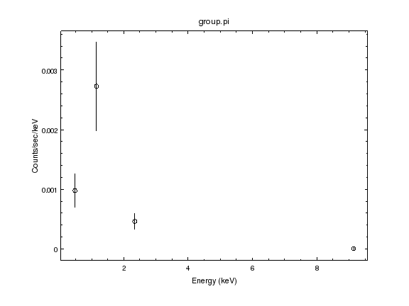
The first look at the source spectrum is not inspiring as there just aren’t that many counts there (which we expected anyway since ∼ 60 counts binned into groups of 20 is only going to produce ∼ 3 bins).
Let’s see what a thermal spectrum looks like. We start by calculating the absorbing column of Hydrogen along the line of site in our Galaxy using the prop_colden command-line tool (rather than the on-line version):
% prop_colden
ASCDS_PROP_NHBASE is not set;
  default assignment to /export/local/ciao-4.4/config/jcm_data has been made.
ASCDS_PROP_NHBASE (for neutral hydrogen column density data) =
  /export/local/ciao-4.4/config/jcm_data
 ----------------- Colden ------------------
 You are now in setup mode.
 Type "c" to enter conversion mode,
      "?" to list setup mode commands,
 or   "q" to quit the program.
The default conversion is from J2000.
Colden[Setup]>: c
NHBASE directory = /export/local/ciao-4.4/config/jcm_data
RA  J2000.0: 7 16 44.3
Dec J2000.0: 37 39 56
------------------------------------------------------------------------------------------
Input coords:  07 16 44.30 +37 39 56.00
Target RA,Dec: 07 13 21.652 +37 45 18.325   (l,b):180.285410    20.869755
Density integrated from   -550.000 to    550.000 km/s
Hydrogen density (10^20 cm**(-2)):   6.98 (Interpolated)
------------------------------------------------------------------------------------------
RA  J2000.0: q
Colden[Setup]>: quit
So the column density is nH = 7 × 1020 cm − 2. Using this, we can construct a model of a thermal plasma - using the X-Spec APEC model - which is absorbed by our Galaxy - using the X-Spec PHABS model, noting that this model has units of 1022 cm − 2 for the nH parameter):
sherpa-6> set_source(xsphabs.gal * xsapec.grp)
sherpa-7> gal.nh = 0.07
sherpa-8> freeze(gal)
sherpa-9> grp.redshift = 0.069
sherpa-10> print(grp)
xsapec.grp
   Param        Type          Value          Min          Max      Units
   -----        ----          -----          ---          ---      -----
   grp.kT       thawed            1        0.008           64        keV
   grp.Abundanc frozen            1            0            5
   grp.redshift frozen        0.069            0           10
   grp.norm     thawed            1            0        1e+24
sherpa-11> fit()
Dataset               = 1
Method                = levmar
Statistic             = chi2gehrels
Initial fit statistic = 3.48061e+11
Final fit statistic   = 0.315056 at function evaluation 74
Data points           = 4
Degrees of freedom    = 2
Probability [Q-value] = 0.854253
Reduced statistic     = 0.157528
Change in statistic   = 3.48061e+11
   grp.kT         1.50713
   grp.norm       1.76513e-05
sherpa-12> plot_fit()
sherpa-13> conf()
grp.kT lower bound:	-0.229734
grp.kT upper bound:	0.407129
grp.norm lower bound:	-4.53886e-06
grp.norm upper bound:	4.84966e-06
Dataset               = 1
Confidence Method     = confidence
Iterative Fit Method  = None
Fitting Method        = levmar
Statistic             = chi2gehrels
confidence 1-sigma (68.2689%) bounds:
   Param            Best-Fit  Lower Bound  Upper Bound
   -----            --------  -----------  -----------
   grp.kT            1.50713    -0.229734     0.407129
   grp.norm      1.76513e-05 -4.53886e-06  4.84966e-06
sherpa-14> plot_fit_delchi()
sherpa-15> print_window('qspec-initial-fit.png')
sherpa-16> quit()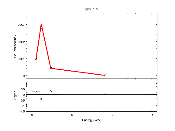
The model (red line) is a good fit to the data, as it should be when there are only 4 data points and 2 parameters to adjust!
So, this initial reduction suggests a gas temperature of ∼ 1. 5 keV, although the errors are large and the analysis has a lot of flaws: for instance
there was no energy filtering applied, which means that data outside the valid detector range (of roughly 0.5 to 7 keV for the ACIS-I array) has been used and could skew the result;
the metallicity was fixed, but it is strongly coupled with the plasma temperature in groups (e.g. see the simulated spectra below);
and the number of counts doesn’t really justify Gaussian errors
but it gives us something to aim at.
What units was that gas temperature in?
X-ray astronomers are quite hapry to talk about a plasma having a temperature of 1.5 keV, even though this is an energy and not a temperature. Why do we do this? Well, it’s because
there is an observational feature releated to this value e.g. see the Wikipedia article on Thermodynamic temperature;
and - perhaps more importantly - the thermal models provided by the X-Spec library use an equivalent energy, rather than temperature, to describe the plasma.
It’s not quite the same reason that particle physicists seem to measure everything as an energy.
Nowadays, rather than having to calculate things manually, we can just ask services like Wolfram Alpha all about 1 keV, and find out that it is equivalent to a temperature of 1. 16 × 107 Kelvin. As a quick comparison, 80 degrees Farenheit is equivalent to 26 meV.
Below we show four simulated spectra, for a thermal plasma with solar metallicities where the temperature ranges between 1 and 10 keV:
% sherpa
-----------------------------------------------------
Welcome to Sherpa: CXC's Modeling and Fitting Package
-----------------------------------------------------
CIAO 4.4 Sherpa version 2 Tuesday, June 5, 2012

sherpa-1> dataspace1d(0.1,10,0.01)
sherpa-2> set_source(xsapec.gas)
sherpa-3> gas.kt = 1
sherpa-4> plot_source()
sherpa-5> log_scale()
sherpa-6> gas.kt = 2
sherpa-7> plot_source(overplot=True)
sherpa-8> set_curve(['line.color', 'orange'])
sherpa-9> gas.kt = 5
sherpa-10> plot_source(overplot=True)
sherpa-11> set_curve(['line.color', 'cyan'])
sherpa-12> gas.kt = 10
sherpa-13> plot_source(overplot=True)
sherpa-14> set_curve(['line.color', 'blue'])
sherpa-15> set_curve('all', ['line.thickness', 1])
sherpa-16> set_plot_xlabel('Energy (keV)')
sherpa-17> set_plot_title('Temperature dependence')
sherpa-18> add_label(0.1, 0.5, '10 keV', ['coordsys',PLOT_NORM,'color','blue'])
sherpa-19> add_label(0.1, 0.4, '5 keV', ['coordsys',PLOT_NORM,'color','cyan'])
sherpa-20> add_label(0.1, 0.3, '2 keV', ['coordsys',PLOT_NORM,'color','orange'])
sherpa-21> add_label(0.1, 0.2, '1 keV', ['coordsys',PLOT_NORM,'color','red'])
sherpa-22> set_label('all', ['size', 20])
sherpa-23> print_window('plasma-temp.png')
sherpa-24> quit()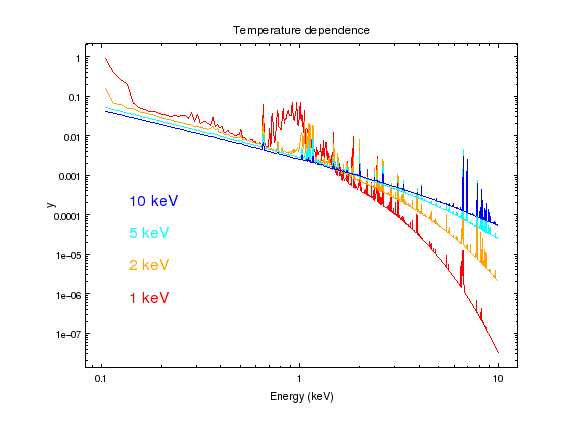
At low energies (below the energy of the plasma), the emission is well approximated by a power law, whereas above this value the emission starts to drop strongly. The temperature of a plasma, when given in energy units, is a measure of this break position. The narrow lines in these plasmas (and not-so-narrow bump just below 1 keV for the 1 keV system) are due to emission from metallic ions in the plasma, which makes temperature and metallicity somewhat hard to disentangle for temperatures around 1 keV. Unfortunately the intrinsic energy resolution of the ACIS detectors is not good enough to resolve these features individually (for that you need to use gratings or an X-ray micro-calorimeter such as flown on Suzaku).
