by Douglas Burke on 2 November 2012
One concern I have when doing a fit - whether to spectra, images, or other data - is how sensitive are the results to the “initial conditions”, that is often thought of as the starting parameter values (which, as I will show below, can change things), but can also be thought of as the energy range used for the analysis (amongst other things).
Scripting things
To avoid too much typing, and keep things repeatable, I have combined yesterday’s analysis steps into the script fit_group.py that defines the Python function dofit with the following signature:
% sherpa fit_group.py
-----------------------------------------------------
Welcome to Sherpa: CXC's Modeling and Fitting Package
-----------------------------------------------------
CIAO 4.4 Sherpa version 2 Tuesday, June 5, 2012

sherpa-2> help(dofit)
Help on function dofit in module __main__:

dofit(elo=0.5, ehi=7.0, fixbgnd=True)
    Fit group.pi with an absorbed APEC model over the
    energy range elo to ehi (in keV) using the Cash statistic.
    The background is modeled as a powerlaw + thermal model
    (both absorbed), fitted separately, then fixed before
    fitting the source (unless fixbgnd is False).
I have added the fit_group.py file to the data distribution on FigShare.
As a check I run it with no arguments, so that it should repeat yesterday’s fit:
sherpa-3> dofit()
***
*** Fix bgnd before source fitting: True
*** Energy range: 0.5 to 7.0 keV
***
read ARF file group.warf
read RMF file group.wrmf
read ARF (background) file group_bkg.warf
read RMF (background) file group_bkg.wrmf
read background file group_bkg.pi
*** Fitting background
Dataset               = 1
Method                = neldermead
Statistic             = cash
Initial fit statistic = 2.61968e+07
Final fit statistic   = 703.056 at function evaluation 343
Data points           = 446
Degrees of freedom    = 444
Change in statistic   = 2.61961e+07
   bgnd.gamma     0.551107
   bgnd.ampl      4.72044e-05
Dataset               = 1
Method                = neldermead
Statistic             = cash
Initial fit statistic = 703.056
Final fit statistic   = 703.056 at function evaluation 290
Data points           = 446
Degrees of freedom    = 444
Change in statistic   = 0
   bgnd.gamma     0.551107
   bgnd.ampl      4.72044e-05
Dataset               = 1
Method                = neldermead
Statistic             = cash
Initial fit statistic = 2.78615e+06
Final fit statistic   = 500.503 at function evaluation 1250
Data points           = 446
Degrees of freedom    = 442
Change in statistic   = 2.78565e+06
   bgnd.gamma     -0.0255636
   bgnd.ampl      2.25478e-05
   gal.kT         0.1954
   gal.norm       0.000100323
Dataset               = 1
Method                = neldermead
Statistic             = cash
Initial fit statistic = 500.503
Final fit statistic   = 500.503 at function evaluation 629
Data points           = 446
Degrees of freedom    = 442
Change in statistic   = 0
   bgnd.gamma     -0.0255636
   bgnd.ampl      2.25478e-05
   gal.kT         0.1954
   gal.norm       0.000100323
Dataset               = 1
Method                = neldermead
Statistic             = cash
Initial fit statistic = 500.503
Final fit statistic   = 496.268 at function evaluation 1568
Data points           = 446
Degrees of freedom    = 441
Change in statistic   = 4.2347
   bgnd.gamma     -0.0738507
   bgnd.ampl      2.10531e-05
   gal.kT         0.196389
   gal.Abundanc   0.022431
   gal.norm       0.00218217
Dataset               = 1
Method                = neldermead
Statistic             = cash
Initial fit statistic = 496.268
Final fit statistic   = 496.268 at function evaluation 707
Data points           = 446
Degrees of freedom    = 441
Change in statistic   = 1.45236e-07
   bgnd.gamma     -0.0738574
   bgnd.ampl      2.1053e-05
   gal.kT         0.196388
   gal.Abundanc   0.0224329
   gal.norm       0.00218218
*** Freezing background
*** Fitting source
Dataset               = 1
Method                = neldermead
Statistic             = cash
Initial fit statistic = 8.13846e+06
Final fit statistic   = 755.432 at function evaluation 306
Data points           = 892
Degrees of freedom    = 890
Change in statistic   = 8.13771e+06
   grp.kT         2.03504
   grp.norm       2.58263e-05
Dataset               = 1
Method                = neldermead
Statistic             = cash
Initial fit statistic = 755.432
Final fit statistic   = 755.432 at function evaluation 279
Data points           = 892
Degrees of freedom    = 890
Change in statistic   = 0
   grp.kT         2.03504
   grp.norm       2.58263e-05
grp.norm lower bound:	-5.95703e-06
grp.norm upper bound:	4.06683e-06
grp.kT lower bound:	-0.529801
grp.kT upper bound:	0.520638
Dataset               = 1
Confidence Method     = confidence
Iterative Fit Method  = None
Fitting Method        = neldermead
Statistic             = cash
confidence 1-sigma (68.2689%) bounds:
   Param            Best-Fit  Lower Bound  Upper Bound
   -----            --------  -----------  -----------
   grp.kT            2.03504    -0.529801     0.520638
   grp.norm      2.58263e-05 -5.95703e-06  4.06683e-06
*** now allowing metallicity to vary
Dataset               = 1
Method                = neldermead
Statistic             = cash
Initial fit statistic = 755.432
Final fit statistic   = 750.072 at function evaluation 494
Data points           = 892
Degrees of freedom    = 889
Change in statistic   = 5.3606
   grp.kT         1.32712
   grp.Abundanc   0.113515
   grp.norm       5.20994e-05
Dataset               = 1
Method                = neldermead
Statistic             = cash
Initial fit statistic = 750.072
Final fit statistic   = 750.072 at function evaluation 423
Data points           = 892
Degrees of freedom    = 889
Change in statistic   = 1.7603e-07
   grp.kT         1.32725
   grp.Abundanc   0.113492
   grp.norm       5.21016e-05
grp.kT lower bound:	-0.225755
grp.norm lower bound:	-1.37811e-05
grp.kT upper bound:	0.402842
grp.Abundanc lower bound:	-0.0887834
grp.Abundanc upper bound:	0.181328
grp.norm upper bound:	1.67819e-05
Dataset               = 1
Confidence Method     = confidence
Iterative Fit Method  = None
Fitting Method        = neldermead
Statistic             = cash
confidence 1-sigma (68.2689%) bounds:
   Param            Best-Fit  Lower Bound  Upper Bound
   -----            --------  -----------  -----------
   grp.kT            1.32725    -0.225755     0.402842
   grp.Abundanc     0.113492   -0.0887834     0.181328
grp.norm 5.21016e-05 -1.37811e-05 1.67819e-05So, the fit results are slightly different to those from yesterday, namely
confidence 1-sigma (68.2689%) bounds:
   Param            Best-Fit  Lower Bound  Upper Bound
   -----            --------  -----------  -----------
   grp.kT            1.29172    -0.171804     0.390972
   grp.Abundanc    0.0932278   -0.0683859     0.183778
   grp.norm      5.19229e-05 -1.53405e-05  1.63004e-05
and it is actually a a slightly-better fit, since the fit statistic here is 750.072 versus 750.483 from yesterday. However, note that the fit results are actually very similar if you look at how different they are in terms of the error (e.g. the temperature difference is ∼ 0. 04 keV, which is a lot smaller than the ∼ 0. 2 keV error), as expected since the difference in the Cash statistic is ∼ 0. 4 (since the difference in Cash statistic can be equated to the δχ2 distribution, this is less than a 1σ change).
Why the difference? Well, yesterday I ended up with a slightly-different set of background parameters because I did not change the gas temperature of the gal component before fitting (so yesterday it started at 1 keV but the script changes this to 0.2 keV). This results in the difference seen above.
I have also created a command doplot that shows the source and background fits (it customises the default Sherpa plot hence the need for a command):
sherpa-4> doplot()
WARNING: unable to calculate errors using current statistic: cash
WARNING: unable to calculate errors using current statistic: cash
sherpa-5> print_window('fit-source-bgnd-0.5-7.0.png')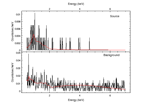
The top plot shows the source fit and the bottom plot the background fit when using the 0.5 to 7.0 keV range.
Expanding the energy range
There is valid ACIS-I data outside the energy range 0.5 to 7.0 keV but I did not use it because
the sensitivity drops strongly outside this energy range so it is unlikely to add much to the analysis;
the background level increases (in particular at higher energies);
the calibration is not as accurate, in particular below 0.5 keV.
However, I am going to try changing the energy range to see what happens; first by using the 0.3 to 8.0 keV range. I have not included the full screen output, as I did above, for these runs, but they are available for download.
First I compare the source spectrum to the sensitivity of the detector, as measured by the ARF:
sherpa-6> plot_source()
sherpa-7> add_axis(Y_AXIS, 1, 0, 1)
sherpa-8> plot_arf(overplot=True)
sherpa-9> set_histogram(['line.color', 'default'])
sherpa-10> set_plot_ylabel('ARF (cm^{-2})')
sherpa-11> current_axis('ay1')
sherpa-12> set_yaxis(['offset.perpendicular', 60])
sherpa-13> log_scale(Y_AXIS)
sherpa-14> current_axis('ay2')
sherpa-15> log_scale(Y_AXIS)
sherpa-16> add_vline(0.5, ['style', 'longdash', 'color', 'blue'])
sherpa-17> add_vline(7.0, ['style', 'longdash', 'color', 'blue'])
sherpa-18> set_axis('all', ['label.size', 18])
sherpa-19> set_plot_title(r'\color{red}Source spectrum  \color{default}ARF')
sherpa-20> print_window('source-arf.png')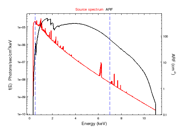
The red line shows the source spectrum (before it enters the telescope) in red, and the effective area (aka ARF) in black. Both are drawn with a logarithmic scale on the ordinate axis. The two vertical lines show the position of the 0.5 and 7.0 keV energies; outside these values the combination of source * ARF drops quickly.
0.3 to 8.0 keV
So, now the 0.3 to 8.0 keV results (done using a new Sherpa session just to make sure that there is no problem with some setting from the previous analysis affecting the results):
% sherpa
sherpa fit_group.py
-----------------------------------------------------
Welcome to Sherpa: CXC's Modeling and Fitting Package
-----------------------------------------------------
CIAO 4.4 Sherpa version 2 Tuesday, June 5, 2012

sherpa-2> dofit(elo=0.3, ehi=8.0)
***
*** Fix bgnd before source fitting: True
*** Energy range: 0.3 to 8.0 keV
***
...
confidence 1-sigma (68.2689%) bounds:
   Param            Best-Fit  Lower Bound  Upper Bound
   -----            --------  -----------  -----------
   grp.kT            1.31973    -0.223513     0.375792
   grp.Abundanc     0.147555    -0.103724     0.201604
   grp.norm      4.76816e-05 -1.36144e-05  1.59915e-05
sherpa-4> doplot()
WARNING: unable to calculate errors using current statistic: cash
WARNING: unable to calculate errors using current statistic: cash
sherpa-5> print_window('fit-source-bgnd-0.3-8.0.png')
sherpa-6> quit()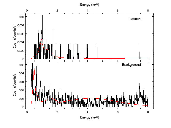
The background can be seen to increase below 0.5 keV and above 7.0 keV, although in reality the change is not huge.
The background model has struggled to account for the new data (the background increase at higher energies should probably be modelled by a separate power law or, in this particular case, a gaussian line, but this extra complexity is not worth it for this analysis); not shown in the output elided above is the fact that the temperature of the gal component is stuck at it’s minimum temperature ( ∼ 0. 1 keV) and abundance (0). Overall the source parameters or their errors are not significantly different.
0.6 to 5.0 keV
% sherpa fit_group.py
-----------------------------------------------------
Welcome to Sherpa: CXC's Modeling and Fitting Package
-----------------------------------------------------
CIAO 4.4 Sherpa version 2 Tuesday, June 5, 2012

sherpa-2> dofit(0.6, 5)
***
*** Fix bgnd before source fitting: True
*** Energy range: 0.6 to 5 keV
***
...
confidence 1-sigma (68.2689%) bounds:
   Param            Best-Fit  Lower Bound  Upper Bound
   -----            --------  -----------  -----------
   grp.kT            1.59163    -0.411918      0.48481
   grp.Abundanc     0.156599    -0.132078     0.261328
   grp.norm       4.6979e-05 -1.25465e-05  1.96818e-05
sherpa-3> doplot()
WARNING: unable to calculate errors using current statistic: cash
WARNING: unable to calculate errors using current statistic: cash
sherpa-4> print_window('fit-source-bgnd-0.6-5.0.png')
sherpa-5> quit()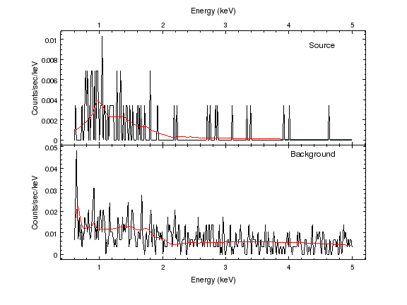
The reduction in energy range means that the single power law component appears to be a better fit to the background
The gal component of the background has an unphysical abundance of ∼ 10 times solar in this fit, but the results overall remain the same. Note that the reduction in the high-energy limit could correspond to the slight increase in best-fit temperature, since there is less of a constraint, but I am probably reading too much into the small changes.
The takeaway message?
It looks like the exact choice of energy range used in the analysis does not significantly influence the results. Now, that’s not to say that this is done and dusted, since I havent’ proved that the emission is actually from a thermal plasma, since I haven’t tried fitting anything else to it!
A powerlaw?
So, does a power law fit as well? I use the same script as above to fit the 0.5 to 7.0 keV data, then change the source model to be an absorbed power law:
% sherpa fit_group.py
-----------------------------------------------------
Welcome to Sherpa: CXC's Modeling and Fitting Package
-----------------------------------------------------
CIAO 4.4 Sherpa version 2 Tuesday, June 5, 2012

sherpa-2> dofit()
***
*** Fix bgnd before source fitting: True
*** Energy range: 0.5 to 7.0 keV
***
confidence 1-sigma (68.2689%) bounds:
   Param            Best-Fit  Lower Bound  Upper Bound
   -----            --------  -----------  -----------
   grp.kT            1.32725    -0.225755     0.402842
   grp.Abundanc     0.113492   -0.0887834     0.181328
   grp.norm      5.21016e-05 -1.37811e-05  1.67819e-05
sherpa-3> set_source(galabs * powlaw1d.plsrc)
sherpa-4> fit()
Dataset               = 1
Method                = neldermead
Statistic             = cash
Initial fit statistic = 2.40818e+07
Final fit statistic   = 751.125 at function evaluation 308
Data points           = 892
Degrees of freedom    = 890
Change in statistic   = 2.4081e+07
   plsrc.gamma    2.63605
   plsrc.ampl     1.11799e-05
sherpa-5> fit()
Dataset               = 1
Method                = neldermead
Statistic             = cash
Initial fit statistic = 751.125
Final fit statistic   = 751.125 at function evaluation 286
Data points           = 892
Degrees of freedom    = 890
Change in statistic   = 0
   plsrc.gamma    2.63605
   plsrc.ampl     1.11799e-05
sherpa-6> conf()
plsrc.gamma lower bound:	-0.274655
plsrc.gamma upper bound:	0.289174
plsrc.ampl lower bound:	-1.545e-06
plsrc.ampl upper bound:	1.69696e-06
Dataset               = 1
Confidence Method     = confidence
Iterative Fit Method  = None
Fitting Method        = neldermead
Statistic             = cash
confidence 1-sigma (68.2689%) bounds:
   Param            Best-Fit  Lower Bound  Upper Bound
   -----            --------  -----------  -----------
   plsrc.gamma       2.63605    -0.274655     0.289174
   plsrc.ampl    1.11799e-05   -1.545e-06  1.69696e-06
sherpa-7> plot_fit()
WARNING: unable to calculate errors using current statistic: cash
sherpa-8> set_curve('crv1', ['line.style', 'solid', 'symbol.style', 'none'])
sherpa-9> set_source(galabs * grp)
sherpa-10> plot_model(overplot=True)
sherpa-11> set_histogram(['line.color', 'blue'])
sherpa-12> print_window('fit-apec-powerlaw-comparison.png')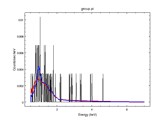
The power-law model is shown in red and the thermal plasma model in blue. The peak in the emission at 1 keV looks to be better fit by the thermal model but it really isn’t clear that we can discriminate between these two models from the spectrum alone.
So, the emission can be adequately explained either as from a hot plasma or from some power-law (non thermal) process. Given that the X-ray emission is from an extended region, rather than a point source, the plasma model is preferred, but one complication is that there could be both processes present - an extended plasma and a power-law component in the central galaxy, since the galaxy does show (faint) radio emission.
As is commonly seen on telescope proposals, more data is needed!
