by Douglas Burke on 1 November 2012
I am going to repeat yesterday’s analysis, but this time fixing the background model before fitting the source region. I have gone back to using the APEC model for describing a thermal plasma, but this should not make much of a difference, as I’ll hopefully show you below.
The data used here - that is the PHA files for the source and background regions together with the relevant response files (ARF and RMF) - is available on FigShare; I had hoped to stick in a fancy FigShare widget but it’s not obvious to me, after looking at the documentation for a whole 5 minutes, how to do that.
% sherpa
-----------------------------------------------------
Welcome to Sherpa: CXC's Modeling and Fitting Package
-----------------------------------------------------
CIAO 4.4 Sherpa version 2 Tuesday, June 5, 2012

sherpa-1> set_stat('cash')
sherpa-2> set_method('simplex')
sherpa-3> load_data('group.pi')
read ARF file group.warf
read RMF file group.wrmf
read ARF (background) file group_bkg.warf
read RMF (background) file group_bkg.wrmf
read background file group_bkg.pi
sherpa-4> notice(0.5, 7.0)
sherpa-5> set_bkg_model(xsphabs.galabs * powlaw1d.bgnd)
sherpa-6> galabs.nh = 0.07
sherpa-7> freeze(galabs)
sherpa-8> fit_bkg()
Dataset               = 1
Method                = neldermead
Statistic             = cash
Initial fit statistic = 2.61968e+07
Final fit statistic   = 703.056 at function evaluation 343
Data points           = 446
Degrees of freedom    = 444
Change in statistic   = 2.61961e+07
   bgnd.gamma     0.551107
   bgnd.ampl      4.72044e-05
sherpa-9> set_bkg_model(galabs * (bgnd + xsapec.gal))
sherpa-10> fit_bkg()
Dataset               = 1
Method                = neldermead
Statistic             = cash
Initial fit statistic = 1.39073e+07
Final fit statistic   = 534.892 at function evaluation 1226
Data points           = 446
Degrees of freedom    = 442
Change in statistic   = 1.39068e+07
   bgnd.gamma     -4.30386
   bgnd.ampl      1.25995e-08
   gal.kT         21.6469
   gal.norm       0.000291383
WARNING: parameter value bgnd.ampl is at its minimum boundary 0.0
sherpa-11> gal.kt = 0.2
sherpa-12> fit_bkg()
Dataset               = 1
Method                = neldermead
Statistic             = cash
Initial fit statistic = 2202.55
Final fit statistic   = 534.891 at function evaluation 867
Data points           = 446
Degrees of freedom    = 442
Change in statistic   = 1667.66
   bgnd.gamma     -4.30352
   bgnd.ampl      1.26065e-08
   gal.kT         21.6469
   gal.norm       0.000291346
WARNING: parameter value bgnd.ampl is at its minimum boundary 0.0
sherpa-13> bgnd.gamma = 0.2
sherpa-14> gal.kt = 0.2
sherpa-15> bgnd.ampl = 4e-5
sherpa-16> fit_bkg()
Dataset               = 1
Method                = neldermead
Statistic             = cash
Initial fit statistic = 874.312
Final fit statistic   = 502.704 at function evaluation 836
Data points           = 446
Degrees of freedom    = 442
Change in statistic   = 371.609
   bgnd.gamma     -0.000141408
   bgnd.ampl      2.33625e-05
   gal.kT         0.188075
   gal.norm       0.000103469
sherpa-17> thaw(gal.abundanc)
sherpa-18> fit_bkg()
Dataset               = 1
Method                = neldermead
Statistic             = cash
Initial fit statistic = 502.704
Final fit statistic   = 497.078 at function evaluation 1501
Data points           = 446
Degrees of freedom    = 441
Change in statistic   = 5.62631
   bgnd.gamma     -0.0689599
   bgnd.ampl      2.11985e-05
   gal.kT         0.191332
   gal.Abundanc   0.0194519
   gal.norm       0.00243217
sherpa-19> fit_bkg()
Dataset               = 1
Method                = neldermead
Statistic             = cash
Initial fit statistic = 497.078
Final fit statistic   = 497.078 at function evaluation 726
Data points           = 446
Degrees of freedom    = 441
Change in statistic   = 2.95145e-06
   bgnd.gamma     -0.0689326
   bgnd.ampl      2.11994e-05
   gal.kT         0.191322
   gal.Abundanc   0.0194594
   gal.norm       0.00243186
sherpa-20> plot_fit_bgnd()
NameError: name 'plot_fit_bgnd' is not defined
sherpa-21> plot_bkg_fit()
WARNING: unable to calculate errors using current statistic: cash
sherpa-22> set_curve('crv1', ['line.style', 'solid', 'symbol.style', 'none'])
sherpa-23> print_window('bgnd-powerlaw-apec-abundance.png')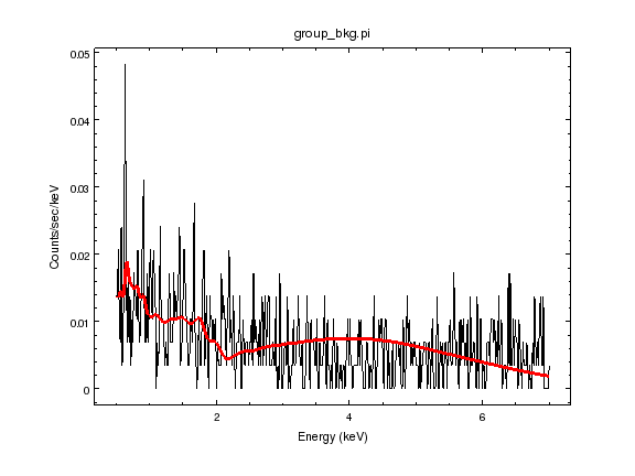
This is very similar to yesterday’s plot, which had a power law with γ = − 0. 03 and thermal plasma with kT = 0. 195 keV for solar abundance. Allowing the abundance to vary has not changed the temperature significantly, even with the abundance falling by a factor of ∼ 50.
As can be seen from the transcript above, I had to fit the background several times, changing the starting point of the fit, to get to the minimum value. This is because when I added in the gal component, the fitting engine decided that it needed to increase the temperature (it started at 1 keV) rather than decrease it. At some level I do not care too much about these components and parameters, since it is intended as a phenomenological model of the background (since the background contamination is small it does not have to be a perfect model of the background, just describe it well). It is, however, nice to get something meaningful; well, for the thermal emission it is, but the power law slope isn’t physical, since the cosmic X-ray background measured by Chandra and XMM-Newton has a slope of γ ∼ 1. 4 at the depth of this observation - e.g. see the background modelling done for XMM-Newton data by Snowden, Collier, and Kuntz, 2004, ApJ, 610, 1182, although I did just note a recent pre-print by Moretti et al. describing a much flatter backgronud spectrum (γ ∼ 0. 1) for a slightly-different energy range using Swift and Chandra data - and I have not included any component to account for the particle background.
I have decided to try fixing this background component before fitting the source since
yesterday’s experiment, in allowing it to vary, did not work well;
and the source region is about 5 percent of the area of the background region and so will not improve on the background constraints.
sherpa-24> freeze(bgnd, gal)
sherpa-25> set_source(galabs * xsapec.grp)
sherpa-26> grp.redshift = 0.069
sherpa-27> fit()
Dataset               = 1
Method                = neldermead
Statistic             = cash
Initial fit statistic = 1.01254e+07
Final fit statistic   = 756.588 at function evaluation 338
Data points           = 892
Degrees of freedom    = 890
Change in statistic   = 1.01246e+07
   grp.kT         1.98496
   grp.norm       2.38852e-05
sherpa-28> fit()
Dataset               = 1
Method                = neldermead
Statistic             = cash
Initial fit statistic = 756.588
Final fit statistic   = 756.588 at function evaluation 287
Data points           = 892
Degrees of freedom    = 890
Change in statistic   = 0
   grp.kT         1.98496
   grp.norm       2.38852e-05
sherpa-29> conf()
grp.norm lower bound:	-6.48428e-06
grp.kT lower bound:	-0.481991
grp.norm upper bound:	4.14228e-06
grp.kT upper bound:	0.514929
Dataset               = 1
Confidence Method     = confidence
Iterative Fit Method  = None
Fitting Method        = neldermead
Statistic             = cash
confidence 1-sigma (68.2689%) bounds:
   Param            Best-Fit  Lower Bound  Upper Bound
   -----            --------  -----------  -----------
   grp.kT            1.98496    -0.481991     0.514929
   grp.norm      2.38852e-05 -6.48428e-06  4.14228e-06
This can be compared to the “quick and dirty analysis” results of
confidence 1-sigma (68.2689%) bounds:
   Param            Best-Fit  Lower Bound  Upper Bound
   -----            --------  -----------  -----------
   grp.kT            1.50713    -0.229734     0.407129
   grp.norm      1.76513e-05 -4.53886e-06  4.84966e-06
and looks like:
sherpa-30> plot_fit()
WARNING: unable to calculate errors using current statistic: cash
sherpa-31> set_curve('crv1', ['line.style', 'solid', 'symbol.style', 'none'])
sherpa-32> 6.7 / 1.069
           6.26753975678204
sherpa-33> print_window('source-xsapec-a1.png')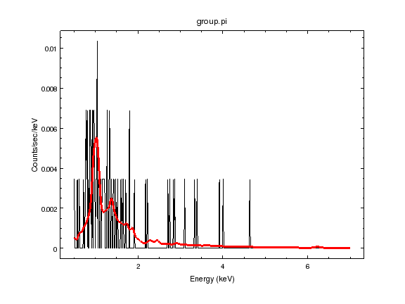
The small blip at around 6.2 keV is the 6.7 keV iron line from the source, redshifted due to the distance of the source, as shown in the calculation above.
sherpa-34> plot_source()
sherpa-35> set_histogram(['line.thickness', 1])
sherpa-36> grp.abundanc = 0
sherpa-37> plot_source(overplot=True)
sherpa-38> set_histogram(['line.thickness', 1, '*.color', 'default'])
sherpa-39> set_yaxis(['offset.perpendicular', 60])
sherpa-40> print_window('source-model-a1.png')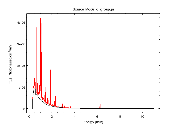
Here we see the source spectrum (red); this can be thought of as the signal that enters Chandra, whereas the fit seen in the previous plot - which blurs out essentially all these lines - is due to the sensitivity and performance of the telescope and the ACIS detector. The black line shows the model when the abundance is set to 0, so the difference is the emission due to the metals in the plasma.
The line at 6.7 keV is due to the presence of metals in the plasma - remembering that we X-ray Astronomers like to split the universe into Hydrogen, Helium, and then lump everything else as a metal - which we see here because the default abundance of 1 (i.e. “solar”) is high. As there is no detected emission at this energy then we may be able to constrain the metallicity in the fit (actually, the whole shape of the spectrum is sensitive to the metallicity at this temperature, as shown in the figure, but the 6.7 keV line is the most obvious individual feature).
I start by re-setting the abundance to 1 - to match the previous fit - thaw it, then fit and calculate the 1-sigma errors using the conf method.
sherpa-41> grp.abundanc = 1
sherpa-42> thaw(grp.abundanc)
sherpa-43> fit()
Dataset               = 1
Method                = neldermead
Statistic             = cash
Initial fit statistic = 756.588
Final fit statistic   = 750.483 at function evaluation 485
Data points           = 892
Degrees of freedom    = 889
Change in statistic   = 6.10447
   grp.kT         1.29172
   grp.Abundanc   0.0932278
   grp.norm       5.19229e-05
sherpa-44> fit()
Dataset               = 1
Method                = neldermead
Statistic             = cash
Initial fit statistic = 750.483
Final fit statistic   = 750.483 at function evaluation 399
Data points           = 892
Degrees of freedom    = 889
Change in statistic   = 0
   grp.kT         1.29172
   grp.Abundanc   0.0932278
   grp.norm       5.19229e-05
sherpa-45> conf()
grp.norm lower bound:	-1.53405e-05
grp.kT lower bound:	-0.171804
grp.kT upper bound:	0.390972
grp.Abundanc lower bound:	-0.0683859
grp.Abundanc upper bound:	0.183778
grp.norm upper bound:	1.63004e-05
Dataset               = 1
Confidence Method     = confidence
Iterative Fit Method  = None
Fitting Method        = neldermead
Statistic             = cash
confidence 1-sigma (68.2689%) bounds:
   Param            Best-Fit  Lower Bound  Upper Bound
   -----            --------  -----------  -----------
   grp.kT            1.29172    -0.171804     0.390972
   grp.Abundanc    0.0932278   -0.0683859     0.183778
   grp.norm      5.19229e-05 -1.53405e-05  1.63004e-05
The result is that the constraints on the metallicity are not strong, but the fit now does prefer a lower temperature. As a check I look at the fit statistic as a function of the temperature and abundance parameters using the region-projection routine (I over-ride the default parameters to better explore the search space for this particular fit):
sherpa-46> reg_proj(grp.kt, grp.abundanc, min=[0.5,0], max=[5.5,3], nloop=[51,51])
sherpa-47> print_window('source-reg-proj.png')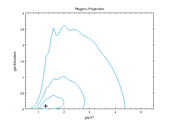
The cross shows the best-fit location and the contours show the 1, 2, and 3 σ confidence contours. Although the parameters are reasonably constrained to 68% (ie the first contour), the constraint is significantly worse at higher confidence levels. The emission is, however, constrained to be > 1 keV to more than 3σ; at least if the metallicity is above 0.3 solar.
Looking at the final fit we get:
sherpa-48> plot_fit()
sherpa-49> set_curve('crv1', ['line.style', 'solid', 'symbol.style', 'none'])
sherpa-50> print_window('source-xsapec.png')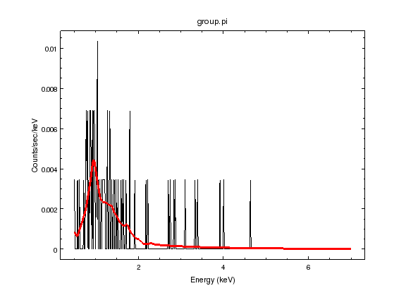
The model looks very similar to the previous fit above, when the abundance was set to solar, except for the lack of the 6.7 keV line and the peak at 1.5 keV is no longer so separated from the one at 1 keV.
Was the background worth bothering with?
In the following I set the background model to 0 and then re-fitting, to see what happens to the source parameters. Given that the background spectrum is significantly “harder” than the source - that is the ratio of counts at high to low energies is larger in the background - I could see that excluding the background would lead to a hotter plasma temperature, as the fit tries to account for the extra high-energy events. Let’s see:
sherpa-51> bgnd.ampl = 0
sherpa-52> gal.norm = 0
sherpa-53> plot_bkg_fit()
The above checks that the model is 0 (note that there isn’t an easy way to clear the background model in Sherpa, at least as far as I am aware, so setting the model to 0 is the easiest work around).
sherpa-54> fit()
Dataset               = 1
Method                = neldermead
Statistic             = cash
Initial fit statistic = 103528
Final fit statistic   = 103526 at function evaluation 423
Data points           = 892
Degrees of freedom    = 889
Change in statistic   = 2.22819
   grp.kT         1.60551
   grp.Abundanc   0.102951
   grp.norm       5.21061e-05
sherpa-55> fit()
Dataset               = 1
Method                = neldermead
Statistic             = cash
Initial fit statistic = 103526
Final fit statistic   = 103526 at function evaluation 406
Data points           = 892
Degrees of freedom    = 889
Change in statistic   = 9.3141e-07
   grp.kT         1.60541
   grp.Abundanc   0.102868
   grp.norm       5.21202e-05
sherpa-56> conf()
grp.kT lower bound:	-0.218989
grp.norm lower bound:	-1.30777e-05
grp.kT upper bound:	0.531437
grp.Abundanc lower bound:	-0.0948807
grp.Abundanc upper bound:	0.213046
grp.norm upper bound:	1.33855e-05
Dataset               = 1
Confidence Method     = confidence
Iterative Fit Method  = None
Fitting Method        = neldermead
Statistic             = cash
confidence 1-sigma (68.2689%) bounds:
   Param            Best-Fit  Lower Bound  Upper Bound
   -----            --------  -----------  -----------
   grp.kT            1.60541    -0.218989     0.531437
   grp.Abundanc     0.102868   -0.0948807     0.213046
   grp.norm      5.21202e-05 -1.30777e-05  1.33855e-05
So the gas temperature has increased, but statistically speaking the change is not significant. The normalisation parameter of the model - i.e. the measure of the amount of gas in the source region - is essentially unchanged, as we would expect, since the background only accounts for ∼ 10% of the emission in the source region.
Why all the re-fits?
In the session above, when I am only concerned about getting close to the best-fit parameters I just call fit or fit_bkg once, but when I want to make sure I am really at the best-fit solution I call the fit twice. Most times the parameter values - and hence best-fit statistic - do not change, which is what we want, but some times there can be a shift if the optimiser - i.e. the algorithm that is attempting to minimize the fit statistic (in this case the simplex, or Nelder Mead, algorithm) - has got caught in a local minimum. If I was after very precise measurements I might change optimiser, or move the parameters slightly and re-fit, just to check that I have the best fit location. I have not done that here, in part because some of the checks I have done whilst writing this page have essentially done this for me (and the page isnt’ exactly light reading as is).
