by Douglas Burke on 31 October 2012
Let’s try a more-detailed analysis of the source spectrum than last time.
We start by loading the data into Sherpa and plotting the un-grouped data, comparing it to he background level (we have to scale by the extraction areas for the comparison; this value is stored in the elegantly-named BACKSCAL variable):
% sherpa
-----------------------------------------------------
Welcome to Sherpa: CXC's Modeling and Fitting Package
-----------------------------------------------------
CIAO 4.4 Sherpa version 2 Tuesday, June 5, 2012

sherpa-1> load_data('group.pi')
read ARF file group.warf
read RMF file group.wrmf
read ARF (background) file group_bkg.warf
read RMF (background) file group_bkg.wrmf
read background file group_bkg.pi
sherpa-2> get_data_plot_prefs()['linestyle'] = chips_solid
sherpa-3> get_data_plot_prefs()['symbolstyle'] = chips_none
sherpa-4> plot_data()
sherpa-5> notice(0.5,7)
sherpa-6> plot_data()
sherpa-7> set_stat('cash')
sherpa-8> plot_data()
WARNING: unable to calculate errors using current statistic: cash
sherpa-9> bplot = get_bkg_plot()
WARNING: unable to calculate errors using current statistic: cash
sherpa-10> norm = get_backscal() / get_backscal(bkg_id=1)
sherpa-11> bx = bplot.x.copy()
sherpa-12> by = bplot.y * norm
sherpa-13> add_curve(bx, by, ['*.color', 'red', 'symbol.style', 'none'])
sherpa-14> set_curve(['line.thickness', 2])
sherpa-15> print_window('source-with-bgnd.png')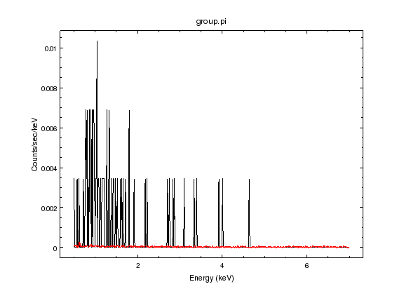
The black line is the source and the red line the background level. The background signal is almost insignificant - earlier I estimated that there are ∼ 5 background events in the 64 events in the source region - except that the background spectrum has a much-different shape to the source. The source emission is concentrated below ∼ 2 keV, whereas the background signal extends across the whole energy range. This is important because we do not want the high-energy events biasing the source spectrum (making it try to account for these photons); one option would be to cut out this energy range from the fit, but we also want to use the lack of counts here as a constraint on the fit.
So now we try to fit the background; note that we have changed to the Cash statistic since we are fitting low-count data (i.e. data for which we can assume a Poission rather than Gaussian distribution). I have chosen to use a Mekal model to account for emission from our own galaxy and a powerlaw model for the other emission (that corresponds to un-resolved X-ray sources and particle background); both are absorbed by gas in the galaxy using the column density used previously:
sherpa-16> plot_bkg()
WARNING: unable to calculate errors using current statistic: cash
sherpa-17> set_bkg_source(galabs.xphabs * (gal.mekal + powlaw1d.bgnd))
NameError: name 'galabs' is not defined
sherpa-18> set_bkg_source(xphabs.galabs * (xsmekal.gal + powlaw1d.bgnd))
NameError: name 'xphabs' is not defined
sherpa-19> set_bkg_source(xsphabs.galabs * (xsmekal.gal + powlaw1d.bgnd))
sherpa-20> galabs.nh = 0.07
sherpa-21> freeze(galabs)
sherpa-22> print(get_bkg_source())
(xsphabs.galabs * (xsmekal.gal + powlaw1d.bgnd))
   Param        Type          Value          Min          Max      Units
   -----        ----          -----          ---          ---      -----
   galabs.nH    frozen         0.07            0       100000 10^22 atoms / cm^2
   gal.kT       thawed            1       0.0808         79.9        keV
   gal.nH       frozen            1        1e-05        1e+19       cm-3
   gal.Abundanc frozen            1            0         1000
   gal.redshift frozen            0            0           10
   gal.switch   frozen            1            0            1
   gal.norm     thawed            1            0        1e+24
   bgnd.gamma   thawed            1          -10           10
   bgnd.ref     frozen            1 -3.40282e+38  3.40282e+38
   bgnd.ampl    thawed            1            0  3.40282e+38
sherpa-23> set_method('simplex')
sherpa-24> fit_bkg()
Dataset               = 1
Method                = neldermead
Statistic             = cash
Initial fit statistic = 3.72332e+07
Final fit statistic   = 532.495 at function evaluation 1147
Data points           = 446
Degrees of freedom    = 442
Change in statistic   = 3.72327e+07
   gal.kT         48.5024
   gal.norm       0.000341969
   bgnd.gamma     -4.61301
   bgnd.ampl      6.99051e-09
WARNING: parameter value bgnd.ampl is at its minimum boundary 0.0
I have just realised that earlier I used the APEC rather than MEKAL model for modelling thermal plasmas; for this data set the difference between these two models should be small.
So, other than suffering several problems in trying to get the model set up, we can see that the fit is not very good (the local emission should have a temperature below ∼ 0. 2 keV, and the power-law slope should be no-where near -5). I have decided to try re-fitting with just the power-law component (since I managed to get this to work earlier in the day):
sherpa-25> set_bkg_source(galabs * bgnd)
sherpa-26> bgnd.gamma = 1
sherpa-27> fit_bkg()
Dataset               = 1
Method                = neldermead
Statistic             = cash
Initial fit statistic = 15457.7
Final fit statistic   = 703.056 at function evaluation 310
Data points           = 446
Degrees of freedom    = 444
Change in statistic   = 14754.6
   bgnd.gamma     0.551107
   bgnd.ampl      4.72044e-05
sherpa-28> fit_bkg()
Dataset               = 1
Method                = neldermead
Statistic             = cash
Initial fit statistic = 703.056
Final fit statistic   = 703.056 at function evaluation 290
Data points           = 446
Degrees of freedom    = 444
Change in statistic   = 1.13687e-13
   bgnd.gamma     0.551107
   bgnd.ampl      4.72044e-05
sherpa-29> plot_fit_bkg()
NameError: name 'plot_fit_bkg' is not defined
sherpa-30> plot_bkg_fit()
WARNING: unable to calculate errors using current statistic: cash
sherpa-31> print_window('bgnd-powerlaw.png')
... on an OS-X machine you will see a lot of scary looking messages now
... that claim problems with the chipsServer such as kCGErrorIllegalArgument
... but these can be ignored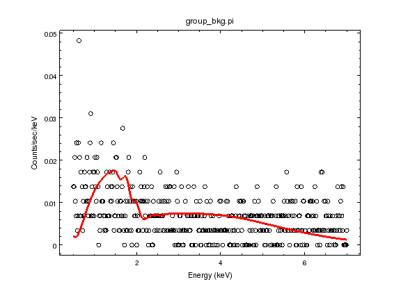
The power law model is in at least the right ball park but it is hard to visualize whether it is a good fit given the data.
I add back in the galaxy emission, tweak the starting temperature to be more realistic, and fit:
sherpa-32> set_bkg_source(galabs * (gal + bgnd))
sherpa-33> gal.kt = 0.2
sherpa-34> fit_bkg()
Dataset               = 1
Method                = neldermead
Statistic             = cash
Initial fit statistic = 946.365
Final fit statistic   = 500.503 at function evaluation 998
Data points           = 446
Degrees of freedom    = 442
Change in statistic   = 445.862
   gal.kT         0.195401
   gal.norm       0.000100314
   bgnd.gamma     -0.0255623
   bgnd.ampl      2.2548e-05
sherpa-35> fit_bkg()
Dataset               = 1
Method                = neldermead
Statistic             = cash
Initial fit statistic = 500.503
Final fit statistic   = 500.503 at function evaluation 629
Data points           = 446
Degrees of freedom    = 442
Change in statistic   = 0
   gal.kT         0.195401
   gal.norm       0.000100314
   bgnd.gamma     -0.0255623
   bgnd.ampl      2.2548e-05
sherpa-36> plot_bkg_fit()
WARNING: unable to calculate errors using current statistic: cash
sherpa-37> set_curve('crv1', ['line.style', 'solid', 'symbol.style', 'none'])
sherpa-38> print_window('bgnd-powerlaw-mekal.png')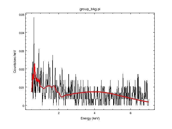
It is not obvious that the “bump” around 3 keV in the model is a good fit to the data, but it gives us something to go with.
Now we have a model for the background we try to fit the source; note that, unlike last time, I have not used the subtract command, which means that the fit we do will automatically include the background component, accounting for the difference in BACKSCAL value which I had to do manually in the first plot above.
sherpa-39> set_source(galabs * xsmekal.grp)
sherpa-40> grp.redshift = 0.069
sherpa-41> print(get_source())
(xsphabs.galabs * xsmekal.grp)
   Param        Type          Value          Min          Max      Units
   -----        ----          -----          ---          ---      -----
   galabs.nH    frozen         0.07            0       100000 10^22 atoms / cm^2
   grp.kT       thawed            1       0.0808         79.9        keV
   grp.nH       frozen            1        1e-05        1e+19       cm-3
   grp.Abundanc frozen            1            0         1000
   grp.redshift frozen        0.069            0           10
   grp.switch   frozen            1            0            1
   grp.norm     thawed            1            0        1e+24
sherpa-42> fit()
Dataset               = 1
Method                = neldermead
Statistic             = cash
Initial fit statistic = 8.13847e+06
Final fit statistic   = 1746.56 at function evaluation 3182
Data points           = 892
Degrees of freedom    = 886
Change in statistic   = 8.13672e+06
   grp.kT         0.0808
   grp.norm       0.000302551
   gal.kT         0.193294
   gal.norm       2.09033e-12
   bgnd.gamma     1.56827
   bgnd.ampl      0.00016626
WARNING: parameter value grp.kT is at its minimum boundary 0.0808
WARNING: parameter value gal.norm is at its minimum boundary 0.0
Oh. I didn’t expect this, namely
the group temperature to be so low (as the warning message points out, this is the minimum temperature for which the XSMEKAL model is valid);
the galaxy emission (as represented by the
galcomponent) is essentially 0 (in fact, all the background components have changed significantly from the background-only fit, which should not happen since the new data included in the fit should not influence the background values that much since the source area contributes hardly any “background” signal).
If I call plot_fit() then the result is not a good fit to the data (since I am using the Cash statistic I can’t just use the statistic value as an indicator of the goodness of fit, unlike the chi-square variants in Sherpa).
Darn it. I had planned to leave with a fit where the group temperature was somewhere in the 1.5 to 2 keV range, as I had managed to get it earlier today when I was exploring the data. So, I’ve done something wrong and it’s not obvious what. Oh well, there’s always tomorrow.
Happy Halloween. I guess I’m showing you the gruesome side of Science, when things don’t go as planned and you run out of time (which, thinking about it, happens most days).
